Software: Python
The goal of this analysis will be to determine which lifestyle factors are most influential in the onset of diabetes.
After our analysis, we can aim to provide recommendations regarding which features are most important in diabetes diagnoses. This is important for two reasons:
It provides further insight on how diabetes can possibly be prevented if patients work to ensure identified features are in optimal condition
If the most influential features are social determinants of health, the task can point out larger-scale inequalities resulting in adverse health impacts
It is important to identify ways individuals can make conscious healthy decisions and systemic factors that make it difficult for minorities to maintain their health so they may be eliminated.
Evaluating the dataset
The dataset had no missing or invalid points.
Conversions:
Binary:
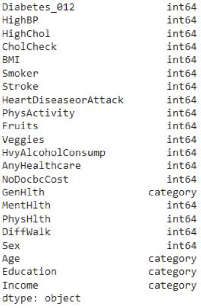
HighBP, HighChol, CholCheck, Smoker, Stroke, HeartDiseasorAttack, PhysActivity, Fruits, Veggies, HvyAlcoholConsump, AnyHealthcare, NoDocbcCost, DiffWalk, Sex
Integer:
Diabetes_012, BMI, MentHlth, PhysHlth
Categorical:
GenHlth, Age, Education, Income
Identifying EDA variables
There are five domains of the Social Determinants of Health:
Economic stability 4. Neighborhood and built environment
Education access + quality 5. Social and community context
Healthcare access + quality
We will consider 'NoDocbcCost', 'Education', 'Income', 'Smoker', and 'HvyAlcoholConsump' as social determinants of health variables, one for each domain.
Diabetic outcomes are represented by the variable 'Diabetes_012'.
We examine the relationship between various features and SDOH using stacked bar charts. We then examine the relationship between SDOH and diabetes using heatmaps.
Relationship between various features and SDOH: HighBP
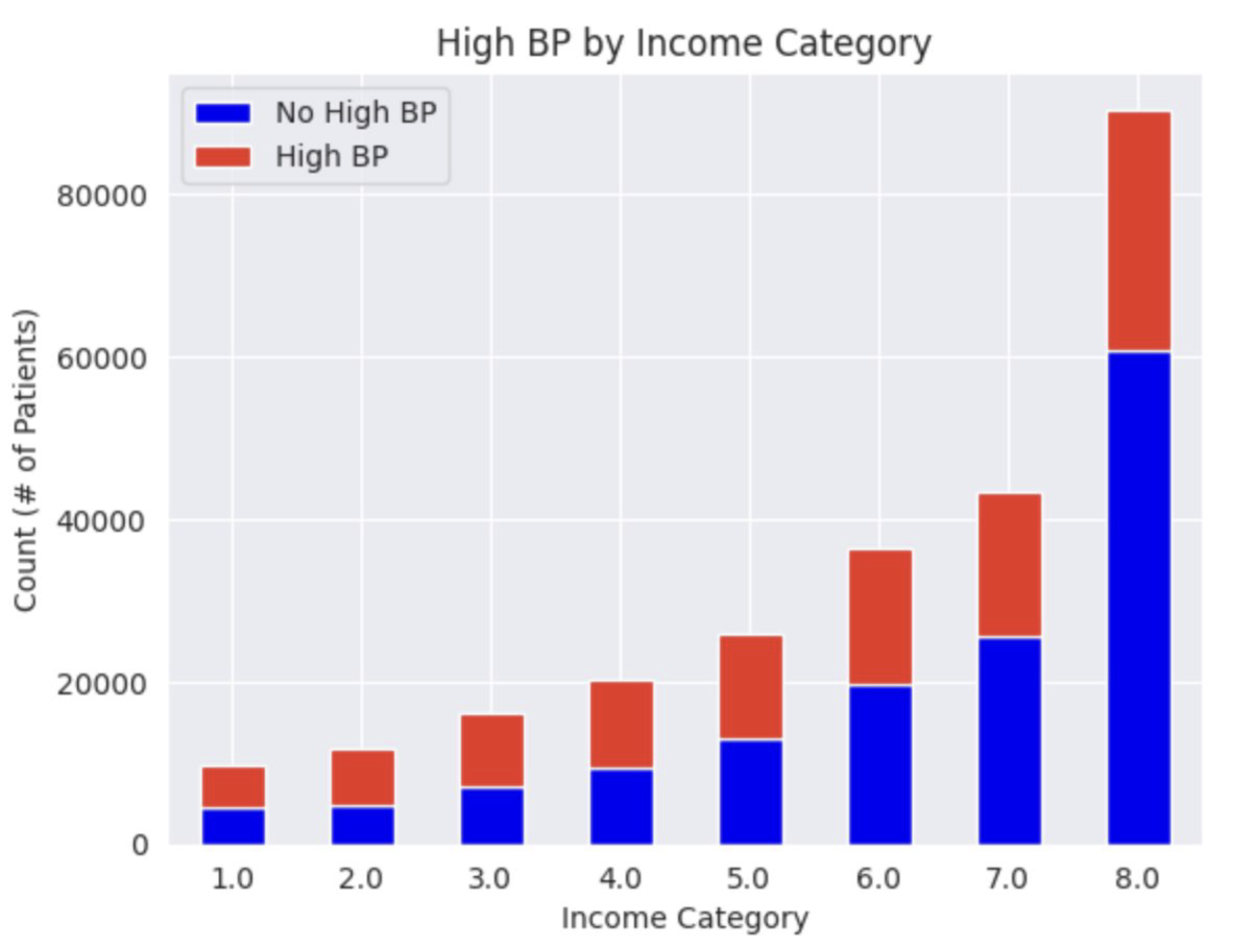
For patients who were less educated (Education = 2 or 3), more patients had high blood pressure than no high blood pressure. For patients who were more educated (Education = 4, 5, or 6), more patients did not have high blood pressure than did. This suggests that as education increases, frequencies of high blood pressure decreases. For low income categories (Income = 1, 2, or 3), more patients were likely to have high blood pressure than no high blood pressure. Where Income = 4, patients seem evenly split between the two categories. For higher income levels (Income = 5, 6, 7, or 8), more patients had no high blood pressure than those who did, suggesting that as income increases, high blood pressure decreases.
Relationship between various features and SDOH: GenHlth
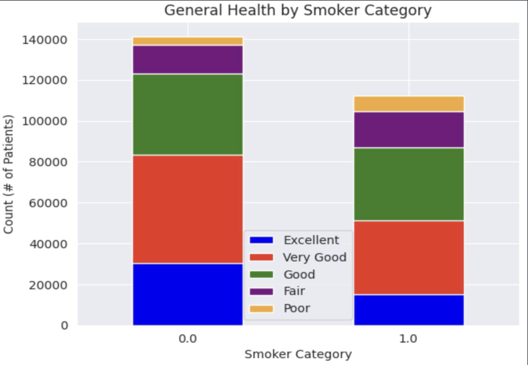
For patients who make anything less than $35,000 per year categories (Income = 1, 2, 3, 4, 5), most patients tend to rate their health as 'Good', followed by 'Very Good', ' 'Fair', 'Excellent', then 'Poor' in most cases (more variability for Income = 1 and Income = 2). For higher income levels (Income = 6, 7, or 8), most patients rank their health as 'Very Good', followed by 'Good', 'Excellent', 'Fair', then 'Poor', although at Income = 6, 'Very Good' and 'Good' ratings were relatively equal. This seems to indicate that as income levels increase, health rankings improve as well. Non-smokers (Smoker = 0) and those who did not consume high amounts of alcohol (HvyAlcoholConsumption = 0) had most patients rate their general health as 'Very Good', followed by 'Good', 'Excellent', 'Fair, then 'Poor', which makes sense given they are not participating in smoking or drinking, known to cause serious health issues. Interestingly, however, smokers (Smoker = 1) mostly rated their health as 'Good' or 'Very Good', followed by 'Fair', 'Excellent', and 'Poor', respectively. There is not enough information to conduct a detailed analysis of heavy drinkers' health ratings, however it is interesting that the 'Very Good' category appears to be most prominent from the limited information we do have.
Relationship between various features and SDOH: Sex
For both patients who could access a doctor when they needed one (NoDocbcCost = 0) and for patients who could not (NoDocbcCost = 1), more patients were female than male. The large number of female patients who could not access a doctor is notable. For patients who make anything less than 35,000 dollars per year categories (Income = 1, 2, 3, 4, 5) and for income level of 6, more patients tend to be female than male. For an income level of 7, there appears to be a somewhat even split between male and female patients. For patients who make $75,000 or more, there seems to be slightly more male than female patients. These findings seem to indicate there are more female patients than male patients in lower income categories, with a more even distribution of sexes as income levels increase.
Relationship between SDOH and diabetes
When comparing 'Education' with diabetic outcomes, most of the patients who were not diagnosed with diabetes (Diabetes_012 = 0) came from education levels greater than 4 (at least a high school graduate).
Of people who were not diagnosed with diabetes, most came from income levels of 6 or higher (make at least 35,000 dollars).
Non-smokers in the data were mostly diagnosed as healthy; smokers were also mostly diagnosed as healthy from a diabetic perspective.
Most patients who were not heavy drinkers were diagnosed as healthy (over 200,000 patients). This also applied to heavy drinkers, though there were fewer diagnosed as healthy (about 13,000 patients).
Performing significance tests
Features of interest:
‘NoDocbcCost’
Was there a time in the past 12 months when you needed to see a doctor but could not because of cost? (0 = No, 1 = Yes)
‘Education’
Education level, scaled by 1-6
‘Income’
Income level, scaled by 1-8
‘Smoker’
Have you smoked at least 100 cigarettes in your entire life? [Note: 5 packs = 100 cigarettes] (0 = No, 1 = Yes)
'HvyAlcoholConsump'
Heavy drinkers (adult men having more than 14 drinks per week and adult women having more than 7 drinks per week) (0 = No, 1 = Yes)
Significance test:
Chi-squared analysis test to determine the strength of relationship between the features of interest and diabetes where p < 0.05 was used as standard to determine a statistically significant relationship.
Utilized scipy.stats library to conduct the chi-square test.
Results
Feature engineering: HealthBehaviorScore
‘HealthBehaviorScore’ was created to encapsulate the following column data:
‘PhysActivity’
‘Fruits’
‘Veggies’
Subtracted ‘HvyAlcoholConsump’ and ‘Smoker’
Results:
Model 1: Random forest design
Features of interest
The features chosen are ‘NoDocbcCost’, ‘Education’, ‘Income’, ‘Smoker’, and ‘HvyAlcoholConsump’.
The target variable is ‘Diabetes_012’.
Class imbalances
Calculated class weights to handle any potential class imbalance.
Hyperparameter tuning
RandomizedSearchCV is used to tune the hyperparameters of the Random Forest. The parameters tuned include n_estimators, max_depth, min_samples_split, and min_samples_leaf.
Best parameters: {'max_depth': 20, 'min_samples_leaf': 1, 'min_samples_split': 8, 'n_estimators': 171}
Model output
Model results
Test set accuracy
0.85
Class interpretations
The class 0 (non-diabetic) has very high precision, recall, and F1-score.
However, for class 1 (diabetic), the recall and F1-score are very low, which means the model is not performing well in identifying the diabetic cases.
The model in the context of the full data set
The results on the full dataset are consistent with the test set, indicating the model generalizes well.
Model 2: SVM
Approach:
Import necessary packages
Sample the data (n = 10,000) using df.sample
Instantiate the SVM model and train using svm.fit
Predict labels for test set and evaluate accuracy using svm.predict and svm.score
Set up parameter grid to test values of ‘C’ and ‘gamma’ using params/np.arange
Use GridSearchCV to tune these two hyperparameters and perform cross-validation (estimator = svm, param_grid = params, cv = 5)
Identify best parameters and best score using .best_params_ and .best_score_
Evaluate mean train/test scores using svm_grid.cv_results_ and diagnose any bias-variance problems
Model results
The accuracy of the model is: 0.846
Classification report:
Best parameters: {‘C’: 1, ‘gamma’: 1}
Best score: 0.8452500000000001
CV results:
The highest mean_test_score was about 0.845, which was coupled with a mean_train_score of about 0.848. The mean training score ranges from about 0.848 to about 0.850, which indicates relatively high accuracy from the model on the training data. The mean test score ranges from about 0.844 to about 0.845, which are quite similar to the mean training scores.
Based on this information, the model does not seem to be over/underfitting the data. The model shows similar mean test scores and mean training scores with a difference of roughly 0.003, suggesting the model was able to perform well with training data and unseen (test) data. Generally, we would say that the model displays low bias and low variance.
Model 3: Logistic regression
Results
The accuracy of the model is: 0.85
Classification report:
Best parameters: {'C': 0.001, 'penalty': 'l1', 'solver': 'liblinear'}
CV results:
The mean_train_score ranged between 0.82 and 0.85 across different parameter settings, suggesting consistent performance during training. The mean_test_score ranged from 0.82 to 0.85, aligning closely with the training scores, which indicates that the model generalizes well to unseen data. The small difference of approximately 0.03 between mean_train_score and mean_test_score indicates low bias, suggesting that the model does not underperform or overperform on training or test data. Both training and test scores have negligible standard deviations, implying low variability in model performance across different folds and suggesting stable predictions.
Model evaluation
1. Random forest
Best parameters: {'max_depth': 20, 'min_samples_leaf': 3, 'min_samples_split': 4, 'n_estimators': 187}
Best CV accuracy: 0.85
2. SVM
Best parameters: {'C': 1, 'gamma': 1}
Best CV accuracy: 0.846
3. Logistic regression
Best parameters: {'C': 0.001, 'penalty': 'l1', 'solver': 'liblinear'}
Best CV accuracy: 0.85
Exploring impacts and bias
Impact:
Individuals at risk of diabetes
Healthcare providers/professionals
Bias:
Potential bias related to protected classes: sex, age, education, income
Created a function to split test data by specific features
Evaluated model performance across different subgroups using accuracy scores and classification reports
This project was the second group project for an asynchronous data science course taken over the summer. Because of this virtual format and the due date falling near the very end of the summer semester, our group faced some difficulties in solidifying meeting times and task distribution as well as generally balancing the project with our other course commitments at the time. One particular challenge we faced was one of our group members feeling overwhelmed with their portion of action items, and a lack of communication prevented my group mates and I from offering assistance prior to the project deadline. This created a mildly stressful project experience, however I have learned the importance of proactive communication and regular check-ins with my group mates throughout the course of the project, not just a few days before the deadline. This project also strengthened my conflict resolution skills as my group mates and I worked with our professor to discuss our submission, a skill that is extremely valuable in group settings.
In thinking about the academic side of the project, this assignment was the culmination of what we had learned in the course, including exploratory data analysis, data cleaning practices, as well as the use of different supervised/unsupervised machine learning models for data analysis. I really enjoyed learning about the different aspects of machine learning in the course, and its exploration of the differences between supervised and unsupervised learning (as well as their use cases and implications).
By analyzing the given dataset using three different models that were new to us (random forest, support vector machines, and logistic regression), this project challenged me as a programmer to not only implement my code correctly for each model, but to also understand what I was doing step-by-step. By reinforcing the differences between models and their insights, I feel more confident in my ability to analyze data using a variety of machine learning models and compare their findings post-execution.


